#319: Testing Trading Algorithms: MACD

Last week we simulated the Bollinger Bands strategy and saw a little improvement over the basic Buy & Hold strategy. This week we build on top of the infrastructure code and add two additional algorithms to our testing plan: MACD and the Moving Average Crossover strategy.

MACD and Moving Average Crossover?

MACD (Moving Average Convergence Divergence) and moving average crossovers are two popular tools traders use to identify trends and momentum in stock prices. A moving average crossover signals buy or sell opportunities when a short-term average crosses a long-term one, helping traders follow the overall market direction.

MACD builds on this idea by measuring the relationship between two moving averages and their momentum, often providing earlier signals and insight into the strength of a trend. These indicators offer different levels of simplicity and depth for timing market entries and exits.

Test the Moving Average Crossover strategy

Thanks to our work in the last week, we can implement the Moving Average Crossover strategy by only focusing on the strategy itself. We need to define the fast and slow average we want to use and can pass different values to our strategy if we work on shorter intervals. The heavy lifting of calculating the moving average is done by Pandas, where we can choose between the ewm() function (Exponentially Weighted Moving) and the rolling() function for a Simple Moving Average). While SMA weights all values equally, EWM gives more weight to recent data points. For more details see this post by whyamit404.

Our strategy implementation looks like this:

class MovingAverageCrossoverStrategy(TradingStrategy):
    def __init__(
        self,
        fast_window=50,
        slow_window=200,
        ma_type="SMA"  # "SMA" or "EMA"
    ):
        self.fast_window = fast_window
        self.slow_window = slow_window
        self.ma_type = ma_type.upper()

    def prepare_indicators(self, df):
        df = df.copy()

        if self.ma_type == "EMA":
            df['MA_fast'] = df['Close'].ewm(
                span=self.fast_window,
                adjust=False
            ).mean()
            df['MA_slow'] = df['Close'].ewm(
                span=self.slow_window,
                adjust=False
            ).mean()
        else:  # SMA default
            df['MA_fast'] = df['Close'].rolling(
                self.fast_window
            ).mean()
            df['MA_slow'] = df['Close'].rolling(
                self.slow_window
            ).mean()

        return df

    def generate_signal(self, df, i, position):
        fast = df['MA_fast'].iloc[i]
        fast_prev = df['MA_fast'].iloc[i - 1]

        slow = df['MA_slow'].iloc[i]
        slow_prev = df['MA_slow'].iloc[i - 1]

        # BUY: fast MA crosses above slow MA
        if (
            position == 0
            and fast_prev < slow_prev
            and fast > slow
        ):
            return "BUY"

        # SELL: fast MA crosses below slow MA
        if (
            position > 0
            and fast_prev > slow_prev
            and fast < slow
        ):
            return "SELL"

        return None

In our test script we only need to replace two lines and keep everything else the same:

# Initialise classes
# strategy = BollingerBandsStrategy(window=20, num_std=2)
strategy = MovingAverageCrossoverStrategy(12, 26, "SMA")
# strategy_name = "Bollinger Bands"
strategy_name = "Moving Average Crossover"

We can run the script to see how this strategy works compared to our Buy & Hold benchmark:

========= Benchmark: Buy & Hold =========
Final value: $13,563.10
Return: 35.63%
Trades:
(Timestamp('2025-01-02 00:00:00'), 138.2721710205078, 'BUY')
(Timestamp('2025-12-30 00:00:00'), 187.5399932861328, 'SELL')

==================================


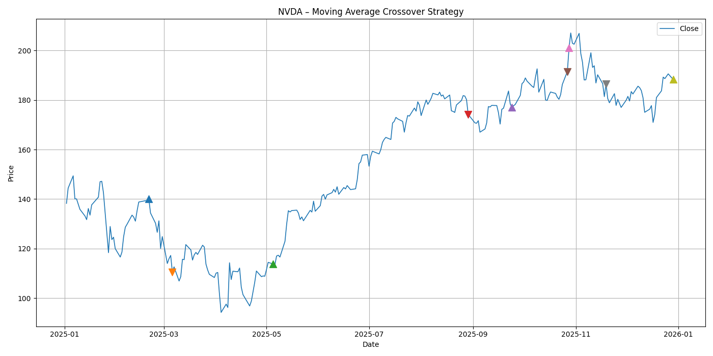
========= Moving Average Crossover =========
Final value: $12,081.39
Return: 20.81%
Trades:
(Timestamp('2025-02-20 00:00:00'), 140.0717010498047, 'BUY')
(Timestamp('2025-03-06 00:00:00'), 110.53976440429688, 'SELL')
(Timestamp('2025-05-05 00:00:00'), 113.79934692382812, 'BUY')
(Timestamp('2025-08-29 00:00:00'), 174.1604766845703, 'SELL')
(Timestamp('2025-09-24 00:00:00'), 176.96014404296875, 'BUY')
(Timestamp('2025-10-27 00:00:00'), 191.47933959960938, 'SELL')
(Timestamp('2025-10-28 00:00:00'), 201.01881408691406, 'BUY')
(Timestamp('2025-11-19 00:00:00'), 186.50961303710938, 'SELL')
(Timestamp('2025-12-29 00:00:00'), 188.22000122070312, 'BUY')

This time we only made a return of 20.81% and lost a lot compared to just buy and hold the stock. On the plot we can see that we participated in the big gain from May to September, but lost on half of the trades:

Test the MACD strategy

To test the MACD strategy, we need again a class that implements the strategy. We use the ewm() function of Pandas to create our signal lines and add them to the DataFrame. We then can run through the data and whenever the lines cross, we get our trading signal:

class MACDStrategy(TradingStrategy):
    def __init__(
        self,
        fast=12,
        slow=26,
        signal=9
    ):
        self.fast = fast
        self.slow = slow
        self.signal = signal

    def prepare_indicators(self, df):
        df = df.copy()

        df['EMA_fast'] = df['Close'].ewm(span=self.fast, adjust=False).mean()
        df['EMA_slow'] = df['Close'].ewm(span=self.slow, adjust=False).mean()
        df['MACD'] = df['EMA_fast'] - df['EMA_slow']
        df['MACD_signal'] = df['MACD'].ewm(span=self.signal, adjust=False).mean()

        return df

    def generate_signal(self, df, i, position):
        macd = df['MACD'].iloc[i]
        macd_prev = df['MACD'].iloc[i - 1]

        signal = df['MACD_signal'].iloc[i]
        signal_prev = df['MACD_signal'].iloc[i - 1]

        # BUY: MACD crosses above signal
        if (
            position == 0
            and macd_prev < signal_prev
            and macd > signal
        ):
            return "BUY"

        # SELL: MACD crosses below signal
        if (
            position > 0
            and macd_prev > signal_prev
            and macd < signal
        ):
            return "SELL"

        return None

To switch our tester to MACD, we again replace two lines:

# Initialise classes
# strategy = MovingAverageCrossoverStrategy(12, 26, "SMA")
strategy = MACDStrategy()
# strategy_name = "Moving Average Crossover"
strategy_name = "MACD"

If we now run the tester, we see the result of the MACD strategy:

========= Benchmark: Buy & Hold =========
Final value: $13,563.10
Return: 35.63%
Trades:
(Timestamp('2025-01-02 00:00:00'), 138.2721710205078, 'BUY')
(Timestamp('2025-12-30 00:00:00'), 187.5399932861328, 'SELL')

==================================


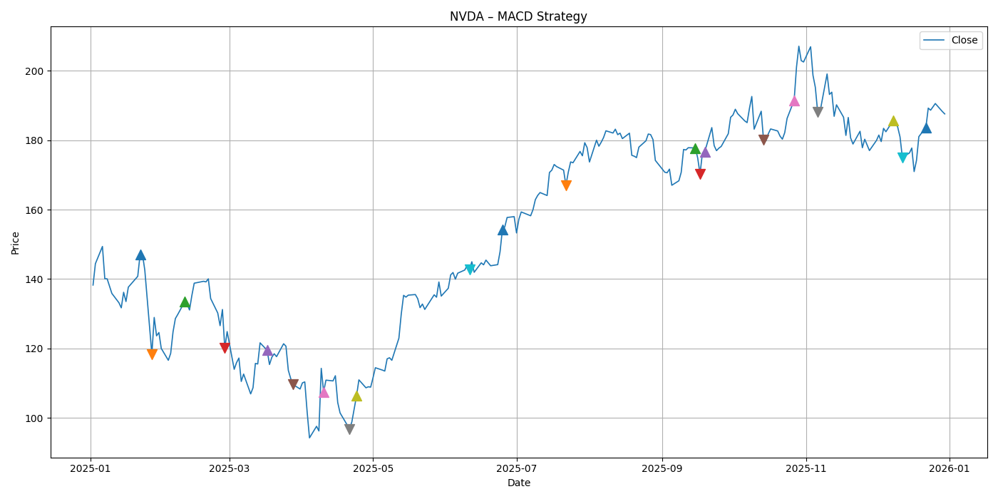
========= MACD =========
Final value: $8,031.25
Return: -19.69%
Trades:
(Timestamp('2025-01-22 00:00:00'), 147.02981567382812, 'BUY')
(Timestamp('2025-01-27 00:00:00'), 118.38761901855469, 'SELL')
(Timestamp('2025-02-10 00:00:00'), 133.53347778320312, 'BUY')
(Timestamp('2025-02-27 00:00:00'), 120.11714172363281, 'SELL')
(Timestamp('2025-03-17 00:00:00'), 119.50830841064453, 'BUY')
(Timestamp('2025-03-28 00:00:00'), 109.65010070800781, 'SELL')
(Timestamp('2025-04-10 00:00:00'), 107.55047607421875, 'BUY')
(Timestamp('2025-04-21 00:00:00'), 96.89241790771484, 'SELL')
(Timestamp('2025-04-24 00:00:00'), 106.41067504882812, 'BUY')
(Timestamp('2025-06-11 00:00:00'), 142.81399536132812, 'SELL')
(Timestamp('2025-06-25 00:00:00'), 154.29270935058594, 'BUY')
(Timestamp('2025-07-22 00:00:00'), 167.01129150390625, 'SELL')
(Timestamp('2025-09-15 00:00:00'), 177.74009704589844, 'BUY')
(Timestamp('2025-09-17 00:00:00'), 170.280517578125, 'SELL')
(Timestamp('2025-09-19 00:00:00'), 176.66015625, 'BUY')
(Timestamp('2025-10-14 00:00:00'), 180.0199737548828, 'SELL')
(Timestamp('2025-10-27 00:00:00'), 191.47933959960938, 'BUY')
(Timestamp('2025-11-06 00:00:00'), 188.0695343017578, 'SELL')
(Timestamp('2025-12-08 00:00:00'), 185.5500030517578, 'BUY')
(Timestamp('2025-12-12 00:00:00'), 175.02000427246094, 'SELL')
(Timestamp('2025-12-22 00:00:00'), 183.69000244140625, 'BUY')

==================================

This strategy would lose us -19.69% and would have been a terrible advice. The reason was that most trades resulted in a loss, as we can see on this plot:

Run everything together

If we only care about the performance of the strategies, we could skip the plot and the trades and just get the summary for each strategy:

strategies = {
    "Bollinger Bands": BollingerBandsStrategy(),
    "MACD": MACDStrategy(),
    "MA Crossover": MovingAverageCrossoverStrategy(12, 26)
}

for name, strat in strategies.items():
    res = tester.run(df, strat)
    print(f"{name:20s} | Return: {res['return_pct']:6.2f}% | Trades: {len(res['trades'])}")

This gives us a nice overview on how the tested strategies would have worked:

Bollinger Bands      | Return:  39.35% | Trades: 6
MACD                 | Return: -19.69% | Trades: 21
MA Crossover         | Return:  20.81% | Trades: 9

Conclusion

We only focused on 3 strategies and one stock to play around. Nevertheless, this tiny set already showed us that trading strategies are not a guarantee for quick success and there is always a risk involved to lose money – even when the stock price mostly goes up during a year. Therefore, do not jump into buying stocks just because someone had a guaranteed strategy. The strategy may be faulty, your implementation of the strategy may have bugs or miss important details, or there may be more unknowns hidden in the market that you cannot know about. Be warned!

With this little experiment our small series on stock market data and trading strategies comes to an end. We now know enough about yfinance to play around on our own, write trading strategies (with or without and LLM) and test them with real data from the past. I hope you enjoyed this topic as much as I did.